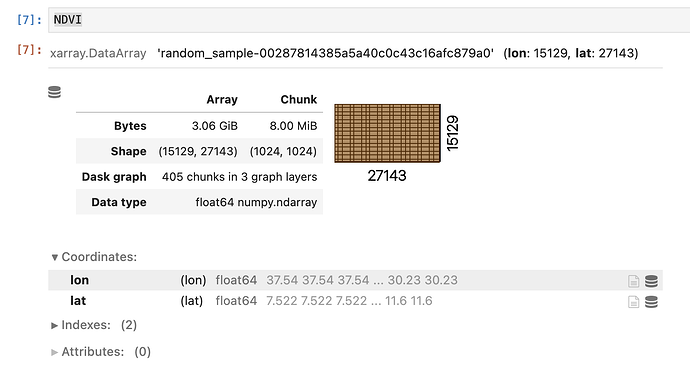
Looking for best strategy to compute quantile over large datasets

[pl.marasco]

I need to compute and assign the 90th percentile of NDVI values grouped accordingly to some ecoregions. To be more clear, assignment has to replace original NDVI values with the corresponded percentiles based on their associated ecoregion.

Bottle neck is the quantile computation, I was not able to find the way to compute in parallel. Is there any other strategy to make this more efficient?
Assignment with delayed approach fails as well but would be nice to achieve that part in parallel as well.

Data

x, y = [27143, 15129]  

# Create dummy data for the coordinates
lat = np.linspace(7.522, 11.6, x)
lon = np.linspace(30.23, 37.54, y)[::-1]

# Create dummy data for the ecoregions
ecoregions = xr.DataArray(
    dask.array.random.randint(1, 1000, size=(y, x), chunks=(512, 512)),
    coords={
        "lon": lon,
        "lat": lat,
    },
    name="ecoregions",
).astype(float)

# Add some nodata values
ecoregions = ecoregions.where(ecoregions < 999)

# Dummy data for the NDVI
NDVI = xr.DataArray(
    dask.array.random.random(size=(y, x), chunks=(1024, 1024)),
    coords={
        "lon": lon,
        "lat": lat,
    },
)

# Add some nodata values
NDVI = NDVI.where(NDVI < 0.99)

Group and percentile computation

# Statck and rechunk the data
stacked_NDVI = NDVI.stack(z=('lat', 'lon')).chunk({'z': -1})
stacked_ecoregions = ecoregions.stack(z=('lat', 'lon')).chunk({'z': -1})

# Group accordingly by eco-regions and compute the 90th percentile for each of them
quantiles = stacked_NDVI.groupby(stacked_ecoregions).quantile(0.9, skipna=True)

Without stacking and rechunking I was not able to achieve a result. With this small sample it’s really slow to compute it.

Assigment

I’ve tested two options and the eager one is the only working. The other inflate like hell in the ram and then workers die.

Eager :

result = ecoregions.copy()
for ecoregion in quantiles.ecoregions:
    result = xr.where(ecoregions == ecoregion, quantiles.sel(ecoregions=ecoregion), result) 

Lazy:

from dask import compute, delayed
# Delayed function to assign quantiles
@delayed
def assign_quantiles_to_eco_unit(ecoregions, quantile_values, eco_unit):
    return xr.where(ecoregions == eco_unit, quantile_values.sel(eco_units=eco_unit), np.NaN)

# Build the delayed computations
delayed_results = [assign_quantiles_to_eco_unit(ecoregions, quantiles, eco_unit) for eco_unit in quantiles.eco_units]

# Compute the results using Dask
results = compute(*delayed_results)

# Combine the results
final_result = xr.concat(results, dim='dummy').max(dim='dummy', skipna=True)

[dcherian]

@pl.marasco

Without stacking and rechunking I was not able to achieve a result. With this small sample it’s really slow to compute it.

I would chunk to a single chunk and then stack (i.e. reshape). It’s identical output but should be substantially more efficient.

In general, the quantile calculation is quite hard. I have been looking in to this on-and-off for a while, but haven’t coded up a solution. Some things I’ve learned so far:

1. In parallel, you can only compute an approximate quantile using “sketch” methods.
2. Some methods (e.g. uddsketch) do come with error guarantees, so the estimates are still scientifically useful.
3. Such approximate methods seem to be “standard” for database implementations (e.g timescaledb)
4. However AFAICT no one has implemented any of these methods for nD arrays, the papers all focus on very long 1D “streams” of data.

dask.dataframe implements the t-digest, so you could try and convert to a dataframe and use that.

As for the assignment, that’s an interesting problem! Particularly so because ecoregions is a dask array. For a numpy array, you can use vectorized indexing (like here). In this case, I would just request a larger memory machine and load ecoregions into memory and construct the “expanded” dataset.

[rabernat]

This is indeed tricky because it’s hard to compute quantiles in a parallel / distributed fashion. The is no simple way to “accumulate” the quantiles from each chunk.

My approach to this problem has always been to transform it into something computationally easier: computing the histogram. From the histogram, you can compute an estimate of the CDF. From this estimate, you can find any quantile you want. (I’d love for a statistician to tell me what’s wrong with this approach; it has always been good enough for our problems.) The nice thing about this is that the histogram is easy to accumulate; you just sum the histogram for each chunk.

In this case, the “groupby” part can be reframed as a joint (2D) histogram of region vs. NDVI. The ability to compute these joint histograms is implemented in the xhistogram package.

Here’s what it looks like.

from dask.diagnostics import ProgressBar
from xhistogram.xarray import histogram
from matplotlib import pyplot as plt

# first align the chunks
ds = xr.merge([NDVI.rename("NDVI"), ecoregions.rename("ecoregions")]).unify_chunks()

ndvi_bins = np.linspace(0, 1, 200)
region_bins = np.arange(1000)
global_hist = histogram(ds.NDVI, ds.ecoregions, bins=(ndvi_bins, region_bins))
global_hist

Now we have a histogram of NDVI for every ecoregion. (NB: I have been a bit sloppy with how I define the bins. Xarray unfortunately still has no notion of finite extents for grid cells, so these coordinates represent the bin centers [n], not the bounds [n+1].)

Computing this is pretty fast for me (5-6 s)

with ProgressBar():
    global_hist.load()

Now we can estimate the CDF by integrating the histogram and plot quantiles

global_hist_normed = global_hist / global_hist.sum("NDVI_bin")
global_hist_cdf = global_hist_normed.cumsum("NDVI_bin")
global_hist_cdf.plot()
cl = global_hist_cdf[:, 1:].plot.contour(levels=[0.5, 0.9, 0.99], colors='k')
plt.clabel(cl)

I’ll leave the final step–interpolating the CDF to specific levels to get the quantiles for each ecoregions–as an exercise for the reader.

---

This is not the most satisfactory or computationally efficient approach to the problem. In particular, it is a bit wasteful of memory–every chunk computes the full 2D joint histogram between NDVI and ecoregions, even if only a tiny fraction of the ecoregions are present. A more sophisticated algorithm would do this reduction in a smarter way.

However, it seems good enough to get the job done.

[mathause]

I found that passing skipna=False does speed up the computation considerably (this of course requires you to know that there are no invalid values) and also using one of the non-interpolating methods (e.g. `method=“lower”) helps as well.

[rabernat]

For curiosity, I tried exporting the data to parquet and running the same query with duckdb.

ds.to_dask_dataframe().to_parquet("ndvi_example/")

import duckdb
query = """
select approx_quantile(NDVI, 0.9), ecoregions from 'ndvi_example/*.parquet'
group by ecoregions
order by ecoregions
"""
duckdb.sql(query)

It took about 5s, on par with the xhistogram approach (but considerably easier to write!) If you are not interested in maintaining the gridded structure of the data, it can be advantageous to just go tabular from the beginning.

Note that doing ecoregions = ecoregions.where(ecoregions < 999) converts the int dtype to float (in order to add NaNs), which may not be ideal here for use as a label.

[dcherian]

@rabernat

From the histogram, you can compute an estimate of the CDF. From this estimate, you can find any quantile you want.

I think there can be accuracy issues because you choose the bins beforehand. “sketches” are basically adaptive histograms that continuously adjust the bins as they ingest new points.

[pl.marasco]

Good point but, unfortunately, we do have nans and time to time can’t be interpolated.

[pl.marasco]

Thanks for all the resources, indeed very useful.

No question about the fact that compute percentile in parallel over a 1D data it’s quite challenging. I remember that long time ago I already had a discussion with Deepak.

However, in this context, the data is grouped by ecoregion, which should “simplifies” the process.
Accordingly to my tests the quantile computation is per se quite fast (~ 1 m ), but the bottle neck is the graph creation (~ 7 m with a graph of ~390 MiB). That also could negatively impact once on a distributed system.

For clarity, here are some constraints that i didn’t mentioned before and I’m working with:

• I require exact values, not an estimation.
• Memory could pose a challenge. This example might seem simple, but the real dataset is significantly larger and that’s why I would love to compute in parallel.
• We need to account for NaN values (skipna is mandatory).
• While ecoregions can be treated as integers, original data are in float32 and that’s why I created the MRE with the same characteristic.

@dcherian Accordingly to my tests change the order of stack and chunk let to a 5% of improvement in term of time. Not that bad not that good; but indeed that’s the correct way to act.

[dcherian]

Is your example dataset missing a time (or some other) dimension? I’m seeing a 3GB array

[pl.marasco]

Not in the MRE; here the dimension is limited to 2d and no other dimension are missing.

Real data are slightly different and, in that case, the NDVI would came out of a mean computed over the time dimension. But again it’s not what has been represented in the example.

[pl.marasco]

@dcherian

For a numpy array, you can use vectorized indexing (like here). In this case, I would just request a larger memory machine and load ecoregions into memory and construct the “expanded” dataset.

@dcherian I did some test but, reusing the MRE you provided I’ve got similar results between the two. Did something changed? (tested under a py 3.11,xr 2023.9.0, np 1.24.4)

anom_current
43.4 ns ± 1.86 ns per loop (mean ± std. dev. of 7 runs, 10,000,000 loops each)

anom_vectorized
42.9 ns ± 1.11 ns per loop (mean ± std. dev. of 7 runs, 10,000,000 loops each)

I’ve tested as well with my data and there is no gain.

[dcherian]

@pl.marasco

I did some test but, reusing the MRE you provided I’ve got similar results between the two. Did something changed?

Yes, I implemented it! So xarray uses that approach.

[dcherian]

This example might seem simple, but the real dataset is significantly larger and that’s why I would love to compute in parallel.

What is the size and chunksize of the big dataset?

[pl.marasco]

short answer:
eco-regions [33897, 36475], chunks (512x512)
ndvi [ 21, 27143, 15129] , chunks (21, 1024,1024)

longer one:
For the eco-regions it’s [33897, 36475] single band f32 Covering the entire Africa. Chunks are not automatically read by the rioxarray and I had to force them to 512x512 (could be that originally data are stored in 256x256).

For the NDVI the situation is slightly different. I’ve only a subset (Tunisia) and the original dataset covers the entire Africa @ 30 meter. For Tunisia it’s [ 21, 27143, 15129] (time, lat, long) f64.
The original dataset it’s composed by 21 single netCDF files and now are stored in a single zarr file with chunks (21, 1024,1024).

The ecoregion has to be forced to the resolution of the NDVI for the overlapping area.

For the NDVI I’ve to compute the median over the entire time dimension and for the first 3 and last 3 years.
Using the eco-regions I’ve to compute the percentile over the 2 aggregated periods.

Up to now, I’m not able to run my MRE on a 64Giga 16Core local machine … try to imagine in a real distributed env.

p.s. the original code is taking leverage of GDAL and Pandas, slow … but it works. Here the point is that I’m trying to advocate the use of Pangeo and the scalability of the process through it.

[dcherian]

Here’s a significantly better way to index instead of using .where a 1000 times (!)

import pandas as pd


def vindex(array, by, by_uniques):
    index = pd.Index(by_uniques)
    if not np.issubdtype(by.dtype, np.int_):
        mask = np.isnan(by)
        by[mask] = -1
    idx = index.get_indexer(by.ravel()).reshape(by.shape)
    expanded = array[idx]
    if not np.issubdtype(by.dtype, np.int_):
        expanded[mask] = np.nan
    return expanded


def blockwise_vindex(array, by, by_uniques):
    array_inds = tuple(range(array.ndim))
    by_inds = tuple(d + array.ndim for d in range(by.ndim))
    return dask.array.blockwise(
        vindex,
        by_inds,
        array,
        array_inds,
        by,
        by_inds,
        by_uniques,
        array_inds,
        meta=array._meta,
        # concatenate all blocks of `array` and then send it over.
        # since `k` is not in the output_inds
        # Thus, `array` should be small enough
        concatenate=True,
    )


# Really we want this
# but https://github.com/dask/dask/issues/8958
# result.vindex[ecoregions_as_integer_indexes]
expanded = ecoregions.copy(
    data=blockwise_vindex(
        array=result.data, by=ecoregions.data, by_uniques=result.ecoregions.data
    )
)
expanded

[dcherian]

@pl-marasco where can I find the actual eco-regions and ndvi datasets that you’re working with.

[pl.marasco]

Sorry for the late answer but I was attending the BiDS’23.

I can share a small sample but I have no idea about the original source. My ultimate goal is to advocate the use of Pangeo so I’ve only partial control over the entire project.
Would this fit your needs? the small sample it’s already enough to demonstrate some criticism in the computation of the quantile.
How could I provide you with the data? may be a private chat would be better to organize all this specific matter.