Interpolation and regridding

hetland · October 17, 2019, 1:14am

After reading some fantastic suggestions for the CMIP6 Hackathon I started to see a common theme emerge for some of the suggestions. At least four of the proposals are focused on interpolation and regridding of model output:

These are all important topics that address common problems in using and analyzing ocean models (and other earth system models as well). The hackathon proposals should be targeted, with achievable goals. I thought it would be good to start a more general discussion about longer term goals, problems, and best practices in regridding and interpolation.

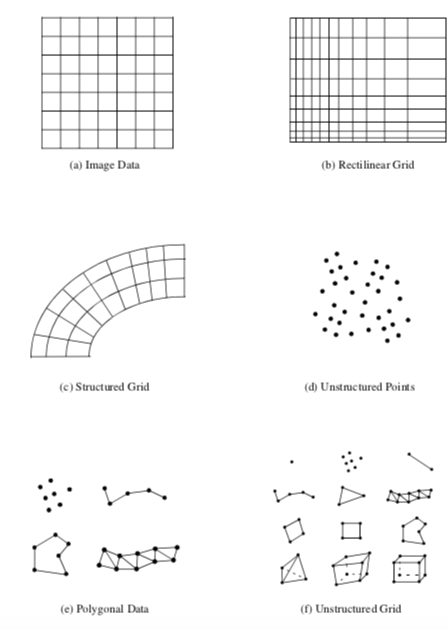
There are three categories of interpolation:

unstructured data mapped to a structured grid
data on a structured grid mapped to unstructured points
data on a structured grid mapped to another structured grid (i.e., regridding)

The four CMIP6 Hackathon proposals are focused on the second and third points. As I see it, these two categories define the two most common use cases for model analysis. The first is used either in creating data-only climatologies (e.g., Levitus) – a career, not an afternoon – or dynamically ‘interpolated’ using a model with some sort of data assimilation. So, if we are interested in model analysis using Pangeo tools, we should focus on the second two.

Interpolation

Interpolating gridded data to random points is straightforward in theory. A common approach is to use Delaunay interpolation, which does not exploit the fact that the original data is on a structured grid. Other algorithms, like quad interpolation (coded up in gridded) can use the information inherent in the grid structure.

A good, general trial case is a glider or profiling float that traces a four-dimensional path through the model field. In my own experience, this is always a frustratingly slow process. It seems the only way to speed this up is to subset the data in a clever way so that interpolation is done only over the data that are needed for a particular timestep.

Re-gridding

There are conservative solutions to the 2D problem, like SCRIP and ESMF. SCRIP, for example, returns a sparse regridding matrix that can be reused, but as far as I know has not been wrapped in a python package. ESMF at least has been translated to an xarray friendly package, xESMF. I’m not sure if the regridding using histograms is conservative, but this might be the most efficient way to translate to a grid that changes in time (e.g., z -> density coordinates).

Though ESMF supports 3D regridding, in practice I have often seen people vertically (1D) interpolate to a z-grid (if not already), then do 2D regridding on each z-level, and finally vertically (1D) interpolate to the desired vertical grid in the target coordinates.

Questions for discussion

What do people do now?
What are the best practices?
What are good-enough practices?
What’s missing?

darothen · October 17, 2019, 4:12pm

Thanks for starting this conversation!

To weigh in a little bit, a common workflow/idiom that I use very frequently with xesmf is the “fit/transform” pattern you often find in scikit-learn and related work. It starts with a “fit” step, where we take a “source” grid and a “target” grid:

import xesmf

source_ds = xr.open_dataset(...)
target_ds = xr.open_dataset(...)

weights_fn = f"{source_grid_name}_to_{target_grid_name}"

# block of code to re-name coords to "lon" and "lat" for simplicity
# ...

regridder = xe.Regridder(source_ds, target_ds, 'bilinear', filename=weights_fn)

Then we just re-use the regridder object in a “transform” step:

regridder = xe.Regridder(source_ds, target_ds, 'bilinear', filename=weights_fn, reuse_weights=True)

regridded_source_ds = regridder(source_ds)

You can wrap these two steps in independent functions and then run them as part of your workflow. For instance, maybe you have a Makefile which has rules to pre-generate the weights files; then you can just use them as a dependency in any of the other steps in your workflow.

In production, I like to cache/save these weights in a dedicated bucket on Google Cloud, and have a function which is basically a look-up table that goes and fetches the weights from the cloud when they’re needed. This way you can cleanly separate the “fit” and “transform” steps in your workflow.

hetland · October 17, 2019, 7:56pm

@darothen, I like your comparisons with scikit learn’s fit/transform pattern. The big advantage in this approach is that you can use a number of different algorithms using the same workflow. Using a different algorithm is as easy as changing one line of code – it’s like magic.

I suppose the same ideas could be used here as well – you could use SCIP under the hood instead of ESMF, and the workflow would be identical. I suspect there are other algoritms that could be included as well.

Also, I think this is 2D -> 2D regridding, based on the lat/lon coords comment. Do you ever need to do 3D regridding?

duncanwp · October 21, 2019, 8:32am

Yes, I think this is an important problem. I think xESMF seems a good approach for regridding but there are still some big gaps when it comes to interpolation.

A long time ago I developed a command line tool based on Iris to try and do this in a general way (https://cis.readthedocs.io/en/stable/collocation.html) but I started splitting this out into separate tools for each problem based on xarrray, see e.g. https://github.com/cistools/collocate.

One problem is that often you have a hyrid dataset with structure in some dimensions and not in others (e.g. structured lat/lon with hybrid pressure levels, or regular time and unstructure lat/lon). Often it’s quickest to interpolate on the structured dimensions before then interpolating the unstructure ones. It’s worth bearing in mind too that the best solution will depend on how many sample points you have compared to how big the data you’re sampling is. If you’re sampling millions of points from a smallish regular grid then it’s useful to sort the points, wheras if you’re sampling a few points from a very large unstrucured grid then sorting doesn’t help.

duncanwp · October 21, 2019, 8:32am

Note, there are a couple of related xarray issues around this: https://github.com/pydata/xarray/issues/486 and https://github.com/pydata/xarray/issues/475

fbriol · November 15, 2019, 9:50am

Hello, I have developed a library which allows perform different interpolations. The library is available here. You can try it with Binder on the github site.

This library has been developed, because I have never found a fast library that allows interpolations on geo-referenced grids. The library is far from perfect, but it meets our needs properly. Today, it allows interpolations to be performed on structured, unstructured grids, binned statistics and fill undefined values.

You can try it and give me feedback.

duncanwp · November 15, 2019, 3:54pm

Cool, I’ll check it out - thanks!

hetland · November 20, 2019, 8:16pm

Though it seems to be pretty straightforward, I think interpolation from quad gridded points to random points is subtle and there is no standard, correct solution yet. This is also being discussed in this pangeo github issue. As for other interpolation needs, it seems ESMF (and xESMF) are regarded as the current standard for gridded to gridded interpolation, and interpolation from random points to gridded points is relatively well understood (e.g., Optimal interpolation for data with errors, Delaunay or cubic spline interpolation for data without).

Interpolation with a grid as random points

The problem in interpolating from quad gridded data to random points is that commonly used methods do not take the information inherent in the grid into account. These methods are basically equivalent to random to random interpolation.

Delaunay interpolation is probably most common, but results can be inconstant, depending on how the quad is split. This effect can be large. Imagine values at the verticies of a quad all zero except for one, which has a value of one. Split one way, the center would have an interpolated value of zero; split the other way, it would be 0.5.

Using a KDTree to find the N closest points, and then interpolating with an inverse distance weights is also problematic, as values can jump suddenly between two nearby query points if they have different furthest points. There is also no guarantee that points will evenly sample across a gradient, causing biases. In practice, jumps and biases can be quite large. This is perhaps the worst method, as seen in this example.

The best method that does not take the native grid into account may be to use some sort of 2D spline approximation, but this is an approximation as the name implies. Overshoots will occur in regions with strong gradients.

Interpolation using information inherent in the grid

Interpolating to a query point from a quad grid requires two steps:

Find the quad in which a query point is located
Use values at the verticies to interpolate

Step one can be done using a number of methods, depending on the grid type. For a rectilinear grid, it is trivial. For a structured (i.e., curvilinear) grid it is more difficult. KDTrees can be used, but some extra logic needs to be applied to find the correct quad attached to the grid vertex nearest the query point. RTrees are similar but potentially faster (e.g., pangeo-pyinterp). However, the fastest method seems to be the CellTree approach (generally described in this paper, and 2d python implementation here).

Step two can be done in 2D with quad interpolation or in 3D with trilinear interpolation. It seems this method could be extended to ND, but might get overly complex with added dimensions. This step is also very fast.

These methods are even easier with a triangle grid, since both steps are more straightforward. Delaunay can be used to find the point in a cell (step 1), though CellTree works for arbitrary polygons, so would also work for triangles. And the interpolation (step 2) is more straightforward, since no remapping needs to be done.

fbriol · December 9, 2019, 3:06pm

I updated the interpolation library to take into account a new interpolator for RTree: Radial Basis Functions. This interpolator allows data to be predicted beyond the data defined in the grids, unlike the IDW interpolator. More details here. This version allows to correctly interpolate the example given by hetland: https://anaconda.org/fbriol/rbf/notebook.

hetland · December 11, 2019, 3:32pm

Radial Basis Functions are fantastic, and I wish they were more commonly used for interpolation. I helped write the scipy rbf subpackage over a decade ago (!), but I think they are still pretty obscure.

One weaknesses of the RBF approach is that it is still an approximation, and can have minima and maxima beyond what are in the original data. This can lead to catastrophic consequences, like generating an unstable water column, or negative salinity in river plume fronts.

Also, since only distance is used for interpolation (orientation between the query point and data points is ignored), there is still the issue of grabbing new points causing jumps, just like with inverse weighted distance. You can see such a jump in the last figure in the notebook posted by @fbriol. Typically this is avoided by using all the data points, as with OI, but this can be very slow to compute, as it requires inverting a matrix the size of the data points squared.

jbusecke · January 17, 2020, 5:38pm

Hey everyone I have been putting together some tools to move between different vertical coordinates in the ocean (but they should be general enough for anything that is defined in a single dimension).

These work with xarray and parallelize nicely with dask for the examples I ran. You can find a test case with several options to change the vertical coordinates here.

I will definitely streamline the interface with a high level wrapper later (right now these need a huge amount of input args), but would love to get some initial feedback before that. Also disregard the rest of the package, its a mess!

leouieda · September 10, 2020, 3:43pm

For radial basis functions and scikit-learn style APIs for interpolation, checkout Verde. The terminology is a bit difference since I’m coming from an applied geophysics and tectonics background but it’s basically the same thing. The library is built around a scikit-learn style API, including spatially blocked operations on scatter data (means, medians, etc), polynomial trends, remove-compute-restore, bi-harmonic splines (the “thin-plate” RBF), and spatial cross-validation. There are plans to add other basis functions, including spherical ones (I’ll probably have a student working on that this year).

An active research project I’m working on is scaling these interpolations out with Dask, but that’s still pretty challenging to get right. We have been able to trade memory for computation time to enable larger datasets on limited RAM but actually distributed fit is tricky.

hetland · September 25, 2020, 6:35pm

I think it will be a hard problem to get interpolation working well with Dask, probably because it’s not simply parallelized. But I’m excited that you are working on this, and hope you succeed.

Every time I think about gridding data, I come across Verde again. I have not yet taken the time to learn it, but think I probably should soon.

bmolero · November 3, 2021, 5:39pm

Hi !

@lrivoire just recently used different libraries to fill NaNs in a map of values organised on an unstructured grid.

He compared your library @fbriol (PyInterp; the functions RBF and IDW) and the Scipy library (the function griddata).

He also confronted different interpolation approaches :

Scipy griddata : nearest neighbour
Scipy griddata : linear (Delaunay triangulation and then barycentric interpolation)
PyInterp RBF : linear
PyInterp RBF : cubic
PyInterp IDW : p=0
PyInterp IDW : p=1

He found that, on the surface he used, the PyInterp library produced better results than the Scipy library, both in terms of statistics (statistics of the difference of the interpolated points with respect to a known truth) and spectrum (computation of the spectrum of the interpolated scene and comparison with the spectrum of the known truth).

The figure below shows from left to right: the true field, the true field with 20% of its pixels randomly set to NaN and the interpolated field using different approaches.

… continues on next comment …

bmolero · November 3, 2021, 5:40pm

The figure below shows the difference between the truth and the interpolated images, only considering the interpolated points : the PyInterp interpolated images seem closer to the truth than the Scipy griddata interpolation.

I can also share the statistics if you want to take a look.