How to correctly convert geostationary satellite data to grid format

Hello everyone,

I am currently working on a project where I need to compare precipitation estimates from a meteorological radar with data from a geostationary satellite.

  • Radar data: Already comes in a grid format with equal pixel height and width. This part is straightforward and easy to handle.

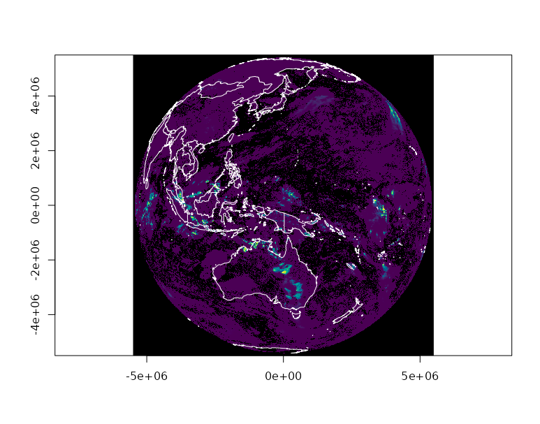
  • Satellite data: Comes in a geostationary projection. From what I understand, this type of data usually needs to be transformed into a regular grid (equal spacing in latitude/longitude or projected coordinates) in order to be compared directly with radar data.

My difficulties:

  1. I am not always sure if I am interpreting the satellite projection metadata correctly. For example, the files include parameters such as:
    Attributes:

    satellite_identifier : HIMA09

    sub-satellite_longitude : 140.7

    centre_projection_longitude : 140.7

    nominal_product_time : 2024-01-07T06:00:00Z

    region_id :HIMA-N

    region_name : HIMA-N; CENTRE=42N 140.7E; SIZE=1044x1896pix

    spatial_resolution : 2.0

    cgms_projection : +proj=geos +coff=2750.500000 +cfac=20466275.000000 +loff=2750.500000 +lfac=20466275.000000 +spp=140.699997 +r_eq=6378.137000 +r_pol=6356.752300 +h=42164.000000

    gdal_projection : +proj=geos +a=6378137.000000 +b=6356752.300000 +lon_0=140.699997 +h=35785863.000000 +sweep=y

    gdal_geotransform_table : [-5.4999955e+06 1.9999983e+03 0.0000000e+00 5.4999955e+06 0.0000000e+00 -1.9999983e+03]

    gdal_xgeo_up_left : -5499995.5

    gdal_ygeo_up_left : 5499995.5

    gdal_xgeo_low_right : 5499995.5

    gdal_ygeo_low_right : -5499995.5

    geospatial_lat_max : 81.04704

    geospatial_lat_min : -81.04704

    geospatial_lon_max : 180.0

    geospatial_lon_min : -179.99997

  2. When I try to reproject or resample the data, I often feel uncertain whether I am aligning the satellite data to the radar grid properly.

  3. I would like to end up with a consistent grid (e.g. 2 km resolution) so I can do pixel-to-pixel comparisons between radar and satellite.

My questions:

  • What is the recommended approach for converting geostationary satellite data to a grid suitable for comparison with radar?

  • Should I first orthorectify the satellite data into a geographic/projection coordinate system, and then resample to match the radar grid?

  • Are there standard tools or workflows (e.g. GDAL, rioxarray, pyresample) that are best suited for this type of reprojection?

  • How can I be sure that the satellite pixels are being mapped correctly onto the Earth’s surface before I compare them with radar?

Any advice, examples, or references would be greatly appreciated!

Data sample available at: https://thredds.nci.org.au/thredds/fileServer/rv74/satellite-products/arc/der/himawari-ahi/precip/crrph/v2.1/2024/01/07/S_NWC_CRRPh_HIMA09_HIMA-N-NR_20240107T060000Z.nc

1 Like

just to note, this is already a regular grid, in the geostationary projection

(using R, where I’m comfortable, first I used gdalinfo on /vsicurl/{url} in order to find the subdataset description)

library(gdalraster)
dsn <- "NETCDF:\"/vsicurl/https://thredds.nci.org.au/thredds/fileServer/rv74/satellite-products/arc/der/himawari-ahi/precip/crrph/v2.1/2024/01/07/S_NWC_CRRPh_HIMA09_HIMA-N-NR_20240107T060000Z.nc\":crrph_accum"
ds <- new(GDALRaster, dsn)
plot_raster(read_ds(ds, out_xsize = 1024, out_ysize = 1024))


chk <- warp(dsn, "/vsimem/new.tif", "EPSG:4326")
dsw <- new(GDALRaster, "/vsimem/new.tif")
plot_raster(dsw)
maps::map(add = TRUE)


That results in these two plots:

Each is just a “raster”, in its own crs, but obviously very different from each other. When you use GDAL to reproject (“warp”, with ‘gdalwarp’ or more recently ‘gdal raster reproject’, or like I do here with the API via a programming language), your job is to specify an output grid, here I only gave a CRS. But, I should give a meaningful region specified by “target resolution” (size of pixels), (OR “target size” (how many pixels)), “target extent” (bounding box in the crs), and the CRS - which can be anything. The data is a regular grid so there’s no extras to deal with, it’s about what is a meaningful choice of rectangular raster space for the work to do next. GDAL will provide heuristics and make these choices for any of size, extent that aren’t specified or implied by inputs.

There’s nothing wrong with the original map projection, that’s as native as it gets and we can zoom in (crop) as we like, use R’s terra or gdalraster, Python’s osgeo.gdal, or rioxarray, or rasterio, or the cli or QGIS, etc - any other CRS choice will be modifying the data, hence a compromise that may or may not be worthwhile.

HTH

here’s a plot with a more meaningful palette, this is a 2km grid (though not equal-area obviously). happy to explore comparison to radar if needed, probably the radar data is more complex in terms of grid? either way, one or the other will be the right “target grid specification” for comparison via least-modification, and I presume the radar is in a more “equal-area” arrangement because it will be local

Can you share a radar file? Getting the bbox, shape, and crs from that will be simple and then it’s a call to gdalwarp (or specified via VRT or some incantation for python). A file can actually be used as the target grid spec too, but then the datatype and contents of the file must be considered of course.

(this is a good example for me if you can share it, it’s related to something I’m writing about) I’m happy to explore whatever is needed to find the right solution

HI @bruno_castro ,

you may have a look into xcube-resampling, if you are happy with doing it in Python and representing the data as xarray.Dataset.

I think @Michael_Sumner is right, both datasets should be raster datasets, and therefore it is a reprojection from one CRS to another.

You can have a look into the function: resample_in_space. An example notebook is given here using this function: https://xcube-dev.github.io/xcube-resampling/examples/resample_in_space_large_example_reproject_dataset/In your case you will need to derive the target_gm from the radar data using the function from_dataset. Your source_gm needs to be derived from the geostationary data. Note that the attributes you showed are not CF compliant. Therefore, you need to explicitly give the CRS. The code would look something like this:

import pyproj
from xcube_resampling.spatial import resample_in_space
from xcube_resampling.gridmapping import GridMapping

gdal_projection = (
    "+proj=geos +a=6378137.000000 +b=6356752.300000 "
    "+lon_0=140.699997 +h=35785863.000000 +sweep=y"
)
crs = pyproj.CRS.from_proj4(gdal_projection)
source_gm = GridMapping.from_dataset(geostat_ds, crs=crs)
target_gm = GridMapping.from_dataset(radar_ds)
geostat_ds_resampled = resample_in_space(
    geostat_ds, source_gm=source_gm, target_gm=target_gm
)

where geostat_ds and radar_dsare xarray.Dataset representing the geostationary and radar datasets, respectively.

Let me know if this work, cause I would be very curious if this is applicable to your use case.

Hello Michael,

thank you so much for the explanation. I managed to reproject to my study area using rasterio.


import numpy as np
import rioxarray
from rasterio.enums import Resampling
from rasterio.transform import from_bounds


src = rioxarray.open_rasterio(
    r'NETCDF:"C:\Users\thomas\Downloads\S_NWC_CRRPh_HIMA09_HIMA-N-NR_20240107T030000Z.nc":crrph_intensity',
    masked=True,
    chunks={"x": 2048, "y": 2048}
)

if "band" in src.dims and src.sizes["band"] == 1:
    src = src.squeeze("band", drop=True)

#bbox in EPSG:4326
lat_min, lat_max = -38.7902, -30.7540
lon_min, lon_max = 141.9084, 149.3825
bounds_4326 = (lon_min, lat_min, lon_max, lat_max)   # (left, bottom, right, top)

#target resolution in degrees
res = 0.02  # ~2 km at equator according to the manual

# Compute shape and transform for the bbox
width  = int(np.ceil((bounds_4326[2] - bounds_4326[0]) / res))
height = int(np.ceil((bounds_4326[3] - bounds_4326[1]) / res))
transform = from_bounds(*bounds_4326, width=width, height=height)

#Reproject ONLY into this bbox grid
dst_bbox = src.rio.reproject(
    dst_crs="EPSG:4326",
    transform=transform,
    shape=(height, width),
    resampling=Resampling.bilinear,
)

dst_bbox=dst_bbox*0.1 #scale factor

dst_bbox.plot()

I checked the manual and set the target resolution to 0.02° (https://www.cr.chiba-u.jp/databases/GEO/H8_9/FD/H08_09_gridded_FD_V02_V20190123_readme_en.pdf). However, I am still unsure whether it is correct to always use a fixed target resolution of 0.02°, or if this value should be recalculated depending on the specific area I am working with.

For the radar data, I don’t have the original polar data. Instead, I am working with a regular grid where pixels have equal height and width. This dataset is a composition of two radars and is provided in EPSG:32755 with a grid resolution of 1000 × 1000 meters. The format is HDF, and I usually handle it by reading with GDAL and then packing the matrix into an xarray dataset, as shown below:

from osgeo import gdal
import xarray as xr
import numpy as np

NAN_VALUE = -499.5

#radar path
radar_path = r'f:\hm428_REINFORM\YARR_HILL_KOMPOSIT_1KM_55S\007_AN2_MJ_Neu_3h_ALLE_mP_mNSW\240107\hd2401070600.scu'
total_bounds = (5707000, 57500, 6588000 + 500, 706500 + 500)  

#Creating lat and lon values based on total bounds
lat_values = range(int(total_bounds[0]), int(total_bounds[2]), 1000)
lon_values = range(int(total_bounds[1]), int(total_bounds[3]), 1000)

#opening and reading radar data
hdf5_file = gdal.Open(radar_path)
radar_array = hdf5_file.ReadAsArray()
radar_array = np.flipud(radar_array) * 0.5 
radar_array[radar_array == NAN_VALUE] = np.nan # replace nan values 


# Xarray dataset radar
ds_radar = xr.Dataset(
    coords={
    'x': (['x'], lon_values),
    'y': (['y'], lat_values),
    }
    )

#Adding radar data
ds_radar['radar'] = (['y', 'x'], radar_array)

ds_radar.radar.plot()

If you’d like to experiment with the original polar data, you can look at one of the individual radars, for example Hillston radar. It has a 360° sweep with 960 pixels per radial, extending from the radar location to the edge of the coverage area. The pixel spacing corresponds to 250 m per gate, giving a total radius of ~240 km. The radar centroid is located at Lat −33.552004, Lon 145.52895 (Australia). The data is also provided in HDF format.

I am packing the files in a link so you have them, the link contains:

  1. Radar composite file (regulargrid_202401070600.scu)
  2. Original radar file (Radar Hillston (polargrid_202401070600)

Link: Unique Download Link | WeTransfer

If you have any question, let me know!

Thank you for the documentation, I will take a look at it and get back to you once I have it done :smile:

Ah, it’s the radar data that is not georeferenced. How did you get this projected bounds above? Neither polar or regular have information afaics, though there is a lon/lat value and some crs info. I don’t know about EPSG:32755, certainly by longitude/latitude it’s in the right zone but this refers to Azimuthal Equidistant (aeqd, not UTM):


what_version_[H5Vol_0.2]=H5rad 2.4
where_height_[m]=144
where_lat_[deg]=-33.551998
where_lon_[deg]=145.52859
where_projdef=+proj=aeqd
where_range=320
where_start_lat_[deg]=6304.7666
where_start_lon_[deg]=248.36517
where_UL_ipixel=1281
where_UL_jpixel=1281
where_xscale_[m]=250
where_xsize=960
where_yscale_[deg]=1
where_ysize=360

That looks like sense can be made of it. Were you provided with those total_bounds from someone? That’s the issue, if you can make a properly referenced grid specification for the radar then gdalwarp(ing) to that would be be the best answer.

I kind of expect that ‘where_lat/lon_[deg]’ is the location of the device (centre of aeqd), and ‘where_start_lon/lat_[deg]’ is the georeferenced offset in the aeqd but that doesn’t check out with the ‘regular’ one having na projdef. The geostat raster is trivial to deal with compared to that, I’d ask for advice about how total_bounds was derived.

I think those lower level radar files are a distraction, the grid you want is in the hd2401070600.scu afaics. So use its extent 5707000, 57500, 6588500, 707000 in ‘-te’, use ‘-ts 1000 1000’ with ‘gdalwarp’, and use ‘EPSG:32755’ in ‘-t_srs’. There are ways to leverage that api via code in various langs, but with rasterio you have to determine the transform (as you showed). Happy to flesh this out if you can share details about hd2401070600.scu

It doesn’t make sense to me to reproject to longlat (EPSG:4326) given what you said above.